The following article and all content provided herein is purely illustrative.
The responsibility for conformity to the specific testing standard being followed falls with the person(s) conducting the test. This document is in no way a replacement for official test protocols as issued by certification authorities.
Introduction
This article outlines a hypothetical Autonomous Emergency Braking (AEB) or Forward Collision Warning (FCW) test conducted using OxTS inertial navigation systems and other products.
Equipment
Hunter Vehicle / Vehicle Under Test (VUT)
RT3003G
Range Hunter
RT Strut
XLAN
Shortwave Radio and Antenna
Target Vehicle / Global Vehicle Target (GVT)
RT3002G
Range Target
RT Strut
XLAN
Shortwave Radio and Antenna or Network Differential Corrections Feature Code
Note: if only stationary targets are required, the tests can be performed using only the Hunter vehicle.
RT Base-S G
Shortwave Radio and Antenna or XLAN
Setup
Base station
Setup the base station in a safe location, ensuring that the GNSS antenna has an unobstructed view of as much of the sky as possible i.e. down to the horizon. If you are wanting to test over multiple days and compare data sets it is recommended that you use the same GNSS antenna location and load the position of the antenna into the base station instead of allowing it to average it's position.
Install RT and RT-Range
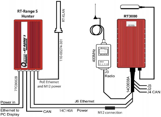
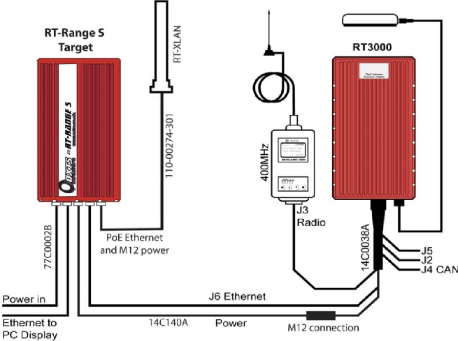
Physically install the RT Strut into the vehicle and mount an RT and Range (Hunter) system on the strut. Choose suitable GNSS antenna locations, ensuring that the antennas are at least 20 cm from the edge of the vehicle's roof and are mounted on a metallic surface. Be sure to place the XLAN and the shortwave radio antennas in positions that do not obstruct the GNSS antennas view of the sky. Ensure all the appropriate connections have been made including antennas, radio, Ethernet and power. Repeat this for the any target vehicles. The wiring diagrams for Hunter (VUT) and Target (GVT) vehicles are shown in figures 1 and 2.
Figure 1: Diagram displaying the connections required to setup the RT units in the VUT.Figure 2: Diagram displaying the connections required to setup the RT units in the GVT. If the differential corrections feature codes have been purchased, the radio is unnecessary.
RT Configuration
Configure the RT(s) with an initial loose configuration (5 deg. and 10 cm tolerances) for orientation and antenna locations, making measurements with the tape measure provided. Be sure to enable and configure lateral and vertical advanced slip. Set your differential corrections format and transmission method also. In most cases you shouldn't need to alter any other settings for the RT.
XLAN (for Multiple Vehicles)
If multiple RTs are being used in combination with RT-Range Hunter and Targets, an XLAN base and one or more XLAN clients are required to communicate between the systems. If the differential corrections feature is enabled, the corrections can be sent via XLAN instead of needing another radio.
Warm up
Go to your test area and use NAVdisplay's warm up template to monitor the RT. You ought to be receiving corrections from the base station, providing that it has finished it's averaging (three minutes by default). This can be checked for by looking at the differential GNSS packet age (differential GPS age), which will be -1 if no packet has ever been received. If all is working correctly this ought to be less than five seconds and your position and velocity modes ought to read "RTK Integer". There ought to be some number of satellites currently being used. A minimum six are required for an RTK Integer level solution, so if you have less than this please ensure that your antenna has an unobstructed sky view and is in an appropriate location, with a good metallic ground plane. The NCOM navigation status should read "Ready to Initialise". You now need to drive the vehicle in a straight line, crossing the threshold velocity of 5 m/s (configurable initialisation speed). This is in order to provide the RT with an initial heading solution under the assumption that the vehicle's heading is approximately equal to the course over ground, when driving straight. For this we take the course over ground at the point your velocity crosses the 5 m/s threshold. Once this has been done you need to begin fifteen minutes of dynamic driving to allow the RT to better estimate it's orientation within the vehicle and the position of the GNSS antennas. We recommend figures of eight of varying radius and velocity as well as some hard acceleration and braking. This process is about getting as large of a range of dynamic stimulus into the RT as possible. Whilst conducting this the warm up template in NAVdisplay will tell you how accurate the RT believes it's measurements are based on it's current estimate of the state of the system. Providing you configured lateral and vertical advanced slip you ought to be able to read the RTs estimation of the heading and pitch misalignment, this can be zeroed out once the warm up is complete using NAVdisplay.
Configuration Refinement
After the fifteen minutes of driving you can commit an improved configuration to the RT in order to provide it a better starting point the next time it is powered on. This is often worthwhile if the same vehicle will be subjected to multiple tests without physically moving the RT or GNSS antennas relative to the vehicle body, however if the vehicle will only be on test on this particular day then this is not necessary. If you do this the unit will reset and a brief warm up will be required again but you ought to see the measurement accuracy values converge much faster than in the previous step.
NAVdisplay Quick Configuration
The quick configuration in NAVdisplay is found under utilities. Before making any changes, make sure to select the option at the bottom of the page that commits the settings to the INS. Here the Slip, Pitch and Roll offsets should be zeroed. This should be done on a flat surface. This is also where the origin and axis of the local co-ordinates of the Hunter RT can be set using it's current position. Configure the x-axis to be along the path between the VUT and the GVT. This will help measure the lateral offset of the vehicles which can help calculate the overlap. The local co-ordinates of the other RT units can then be set by reading them directly from the Hunter RT.
Range Configuration
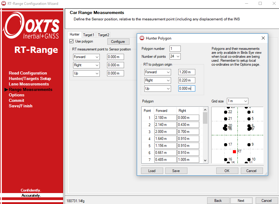
To configure the Hunter, select the IP address of the RT that is being used in the VUT. If mobile targets are being used as the GVTs, select the number of targets and set their IP address’. If fixed point targets are being used, set their locations. These can be set using the current position of the Hunter RT. Set up the polygons by inputting the measurements of the car. Make sure to place the RT unit in the polygon properly. There is a polygon creation tool on our support website. There are also some standard NCAP test dummies here.
Figure 3: Window in the RT-Range configuration showing an example polygon.
If you are using a fixed point target, then you should use the same polygon for both the GVT and the VUT. This can be done through the save and load function in RT-Range config wizard. For the sensor point location, use the front centre of the bumper of the VUT or if multiple sensor points are enabled then place them where the car has its front sensors. For the GVT use the back centre or on the back sensors. It is important to enable the local coordinates in the option page and read them directly from the Hunter RT. Finally, drive away from the target before slowly approaching it again from behind. Try to get close to the target (fixed or mobile) so that the sensors points of the VUT and GVT are almost touching and then zero the longitudinal and lateral offsets using the RT-Range quick config.
CAN Acquisition
RT range output can be done over CAN bus if required. It is enabled in the options page of the RT range software. The navigation CAN messages from target vehicles are output by the RT-Range Hunter. This allows the acquisition system in the hunter vehicle to collect all the measurements from the hunter vehicle and the target vehicles together. Select only the messages needed in the RT range software so that the can bus is not overloaded. More details can be found in this article.
Test Execution
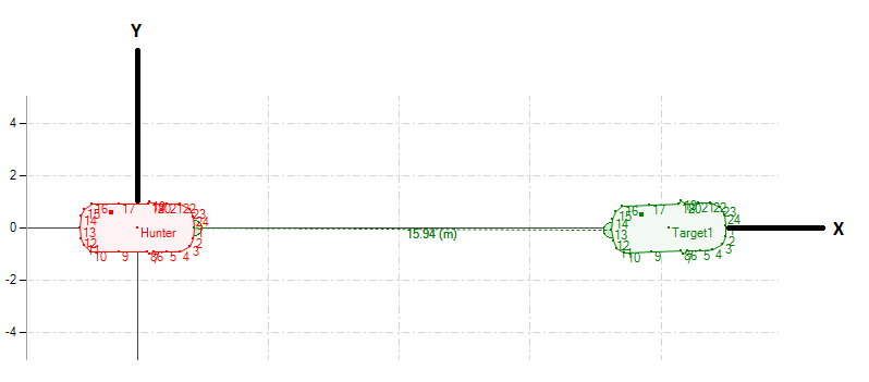
Many AEB and FCW testing protocols specify that both the VUT and GVT positions are controlled laterally to follow a test path. This is often taken as the centre of the lane in which the test is to be conducted. This path can be tracked using driver inputs or robot control. If robot control is to be used then the path can be defined in the robot control mechanism. If the path is to be tracked with by a driver then then it is recommended to setup a local coordinate grid both in the RTs and RT-Range Hunter, as described in the setup section. This will allow the driver to track lateral deviation from the test path in real time and post process. The local coordinate origin should be placed in the centre of the lane where the test is to be conducted, with the X axis running parallel to the lane, such that lateral deviation from the test path will be given as a none zero Y position. This is also useful for calculating the percentage overlap between the VUT and GVT.
Figure 4: This is an example of the test route being aligned with the x-axis of the local co-ordinates of the Hunter.
Boundary Conditions
Test validity usually depends on boundary conditions pertinent to the test being upheld. These will vary depending on the test protocol and specific test being carried out.
Some typically tracked boundary conditions are given below.
Speed of VUT
Speed of GVT
Lateral deviation from test path for VUT
Lateral deviation from test path for GVT
Relative distance
Yaw rate of VUT
Yaw rate of GVT
Steering wheel velocity
Equipment Accuracy
Test protocols will also specify the minimum accuracy of the equipment that ought to be used. It should be noted that the accuracy of an RT is dynamic as the Kalman filter estimates the state of the system and it's relationship to the GNSS antennas and vehicle body over time. However, the RT also reports it's own estimation of measurement errors, so users can monitor the equipment accuracy throughout the test ensuring test validity is upheld. It is useful to think of the equipment accuracy values as another set of boundary conditions to monitor. The exception to this is direct inertial measurement (acceleration and angular rates) which are given in a "raw" state in order to maintain low latency output.
Some measurement accuracies of interest are given below.
VUT and GVT Speed Accuracy
VUT and GVT Position Accuracy
VUT and GVT Yaw Rate Accuracy
VUT and GVT Longitudinal Acceleration Accuracy
VUT Steering Wheel Velocity
Steering Wheel Angle
Brake Pedal Stroke
Accelerator Stroke
Brake Temperature
End of test conditions
This will, again, depend on the specific test protocol, but end of test will often be triggered when particular conditions are met. Typically if the VUT comes to rest or the velocity of the VUT is less than that of the GVT (VUT and GVT begin to diverge) or if contact occurs between the VUT and GVT the test will be over.
Real Time Monitoring and Data Acquisition
All of the previously mentioned measurements and boundary conditions can be monitored and logged in real time over Ethernet using NAVdisplay. There is an AEB testing NAVdisplay template attached to this article that contains most of the typically tracked measurements and their accuracies, including lateral deviations from the axis. The Real-Time Display in the RT-Range software can also be used to check the test has been setup correctly and to monitor the range measurements.
During the test, the test and save function should be used. This can be done through NAVdisplay or the RT Range software. There is a test template available for this which has start of test and end of test conditions, for example, start data recording when time-to-collision (TTC) < 4 seconds and finish data recording when VUT speed < GVT speed or VUT speed < 0.
If you are utilising a data acquisition system we would recommend decoding our Ethernet output for the lowest latency and also to free up more CAN bus capacity for monitoring the vehicle systems and other instrumentation. All of the RT and RT-Range Ethernet data comes time stamped with GPS time in every packet. This means that all data from any OxTS devices is easy to synchronise, whether the data is logged or post processed. If you have CAN to capture either from the vehicle or other instrumentation up to twelve messages can be acquired by each RT. This is then rebroadcast in the Ethernet stream as well as logged internally for post processing later.
If you wish to syncronise CAN logged by a data acquisition system with OxTS data, be it real time or post processed, the best way to do this is to have an RT or RT-Range output the RT GPS time as a high priority CAN message to be logged alongside your other CAN, giving you the same time base in both your Ethernet data and also your logged CAN.
Alternatively, you could set the RT-Range to output all measurements as CAN to be logged by a third party data acquisition system, however due to the nature of CAN and any other communication that maybe taking place on the same bus latency on these signals cannot be guaranteed and the more messages put on the bus the worse this becomes.
Performing the Test
The specifics of the test will differ slightly depending which board protocol you are following but the general test goes as follows: After setting up the base station, configuring the units and warming up, set local coordinates and zero offsets. Line VUT and GVT up along the x axis. Start the data logging if no start condition has been set. Drive at the set speed towards the GVT. Monitor the units using the AEB testing NAVdisplay template. Stop the data logging when end conditions have been met. Repeat for all combinations needed.
Post Processing
Retrieving the Raw Data:
Access the raw data from RT units by opening FileExplorer whilst connected to the same network as the units (e.g. via ethernet). In the search bar at the top, type “ftp://” followed by the IP address of the Hunter RT. Copy the RD files on to the PC into an appropriate folder. Do this process again for the Hunter, this time copying the range config file. Repeat this process for any Target units that were used. It is useful to have access to the RD file as well as the RCOM/NCOM/XCOM files created during the test, as it allows one to post-process the data with different settings if necessary.
Post-Processing the Raw Data (RD to RCOM):
Use the ‘RT Post-Process Wizard’ to create an NCOM file. Load the ‘RT-Range Post-Processing Wizard’ and select the NCOM file that was created. In the ‘Read Configuration’ section, load the range config file that was copied from the Hunter. If a map was created and used during the test, then load the map file in the ‘Lane-Tracking Mode’ section. In the ‘Target Files Setup’ section, any fixed points that were used should already be displayed. If a Target and RT system was used to provide a moving target for a CCRm or CCRb test, then a ‘Mobile Target’ will need to be added and the NCOM file from the Target RT needs to be loaded. The measurements in the ‘Range Measurements’ section should be already be filled from the configuration file. In the ‘Options’ section, ‘Local Co-ordinates’ should be enabled. Check that these co-ordinates match those used during the tests. Click the next button and an RCOM file will be created. It isn’t necessary to select fields and export a csv file as this can be done later using NAVgraph.
Post-Processing the RCOM file:
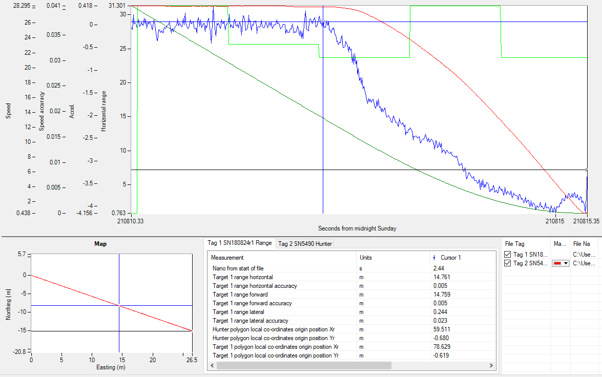
Download the attached 'aebNAVgraphtemplate' and save it to C:\ProgramData\OxTS\NAVgraph\Layout. Open the RCOM file (either produced during the test or by post-processing the raw data) using NAVgraph. In the bottom right-hand corner, use the drop-down menu to select ‘aebNAVgraphtemplate’. Some example test data is shown in figure 5 using this template.
Figure 5: The NAVgraph AEB test template with some example data.
The measurement table has two tabs. One will contain the data from the Hunter RT. These measurements are all related to the movement and orientation of the VUT. The other tab contains all the Range measurements. These are the positions of the VUT and the GVT in the local co-ordinate frame that was setup during the test as well as the distance between them. More measurements can be added to each list. Simply right-click in the table, select ‘Configure Table’ and press the ‘Add Measurements…’ button in the ‘Cursor Table Configuration’ window. The measurements displayed on the graph will be the horizontal range between the VUT and GVT as well as the horizontal speed, horizontal speed accuracy and forward acceleration of the VUT. These can be changed, and more measurements can be added. This is done by right-clicking on the graph and selecting ‘Configure graph’.
RCOM to CSV:
To perform more quantitative analysis, right-click on the graph, hover over 'Export' and select 'CSV file format.’ Tick the ‘Export to a single file’ box. The exported file will contain all the data from the fields in the measurement table and can be opened in Microsoft Excel or used by another program to perform further analysis.
Example Results
This procedure has been followed to perform an AEB test (CCRs) using a single vehicle equipped with a Hunter and an RT3003G. A fixed point was setup to be used as the GVT. The local co-ordinates were setup such that the x-axis was aligned with the test route, as shown in figure 4. The test and save function in NAVdisplay was used. The start condition was the time-to-collision falling below 4 s. The stop condition was horizontal speed reaching 0 m/s. A driver then performed the test at 20, 30 and 40 km/h. The test was also performed with various lateral overlap values at 30 km/h.
Impact Speed:
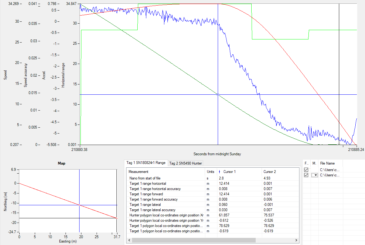
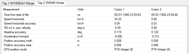
Figures 5 and 6 show data taken from two tests performed at 30km/h with 100% overlap. In figure 5, the horizontal range never passes 0 before the end of the test. Since the test ends when the VUT becomes stationary, this signifies a pass as the vehicles never collided. In figure 6, cursor 2 shows where the horizontal range passes 0, indicating a failed test. The impact speed can found easily by looking at the Hunter tab in the measurement table and reading off the horizontal speed value for cursor 2. This is shown to be 5.66 km/h in figure 7.
Figure 6: This NAVgraph displays shows the data from a failed test.Figure 7: The Hunter tab in the measurements table shows that the impact speed in this test was 5.66 km/h.
Lateral Path Error and Lateral Overlap:
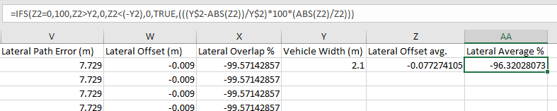
One possible example of using the .csv file is calculating the lateral overlap between the VUT and the GVT. To calculate the lateral overlap, only the ‘Hunter polygon local co-ordinates origin Yr’ (Y value of the VUT) and the ‘Target 1 polygon local co-ordinates origin Yr’ (Y value of the GVT) columns will be needed. The lateral path error is simply the sum of the absolute Y values of the VUT and GVT, due to the way in which the x axis of the local co-ordinates has been setup. The lateral offset between the two vehicles is simply the difference between the Y values of the VUT and the GVT. To calculate the overlap percentage, the VUT width will be required. A formula for calculating the lateral overlap percentage is shown below in an example Excel workbook.
Figure 8: Example Excel workbook showing the formula used to calculate the lateral overlap percentage.
This formula works using a series of if statements: If the lateral offset is 0 then the overlap is 100%. If the lateral offset is greater than the width of the Hunter vehicle (for positive offset, less than for negative offset) then there is no overlap. Else the overlap should be calculated. The last term in the formula is used to give the overlap percentage the same sign as the overlap (and is the reason that the 0 offset case had to be dealt with separately, to avoid errors caused by dividing by 0).
Filtering the Data:
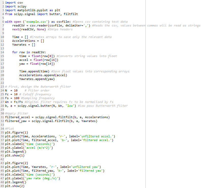
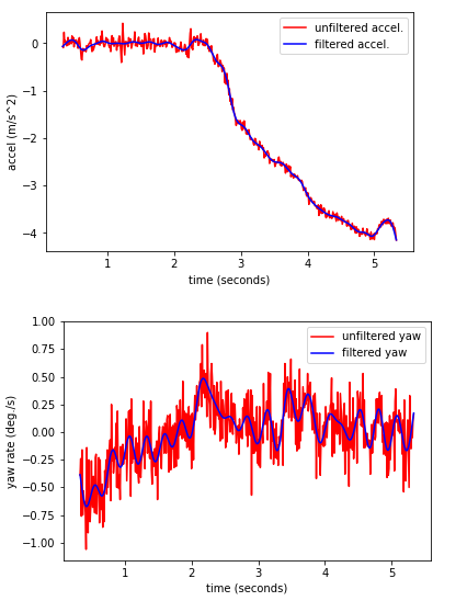
There is an option in NAVconfig to apply a selection of filters to the angular and linear acceleration and specify properties like the cut-off frequency. If the specific test board being used requires different filters, or different measurements to be filtered, then a short program can be written that reads the measurements from the .csv file and applies the filter. The example below is a simple python script that applies a Butterworth filter to the forward acceleration and ISO e.f.s yaw velocity. The figures produced by this script show the filtered and unfiltered measurements plotted on the same graph. These are shown in figure 10.
Figure 9: An example of how to apply filters to the measurements during post-processing. Figure 10: Plots produced by the example Python script showing the filtered and unfiltered acceleration and yaw velocity measurements.
If you have further questions around the application of OxTS products for conducting specific scenarios please contact support@oxts.com

Comments
0 comments
Please sign in to leave a comment.